How to create a Pivot Table in Excel
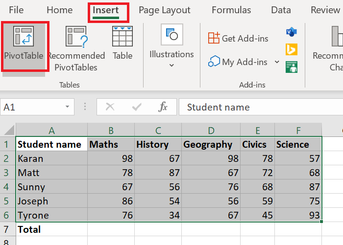
First of all, you would need a set of data arranged across rows and columns. Eg. The lists of marks scored by students in various subjects. Assume that you need the total of each student’s mark in all the subjects in the last row. You could use a formula and pull it across the cells using the Fill function, but that would be useful only till the rows and columns are not changed. To create a pivot table, the procedure is as follows: The case mentioned above is a generic one where you need the sums of values in a single column in the last row. In case you wish to make modifications, please use the option for recommended Pivot Tables under the Insert tab. Read: How to change the color of the Excel worksheet Tab.
How to create a Pivot Chart in Excel
Once you have created the Pivot Table, you can make a Chart of it. The procedure is as follows: Select the range of cells across the Pivot Table. Go to Insert and under the section for Charts, select Pivot Chart. Select the type of chart you wish to use and hit OK. Let us know if you have any doubts in the comments section. Now read: How to use SUMIF and SUMIFS Functions in Microsoft Excel.