How to make a Pie Chart in Excel
In this article, we would consider the Hierarchical Sunburst chart as a type of pie chart, though the procedure for adding it is a little different. The procedure to create a pie chart for data spread across 2 columns only is simple. Select the data across the 2 columns in question.
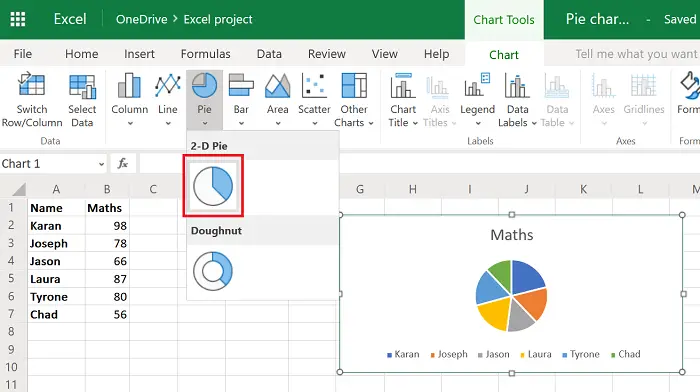
Click on Insert > Pie Chart.Then select the 2-D pie chart.
A larger view of the 2-D pie chart is as follows:
In case you select data across more than 2 columns while using the 2-D pie chart, the chart will ignore entries beyond the first 2 columns.Similar is the case for a hierarchical sunburst chart.Select the data across the 2 columns in question.Click on Insert > Other Charts > Hierarchical > Sunburst.
A larger view of the hierarchical sunburst chart is as follows: The chart will appear similar to the pie chart of your Excel sheet, but the values would probably be mentioned inside the pies.
Make a chart with data spread across multiple columns in Excel
Ideally, a pie chart isn’t the best option for those dealing with multiple columns. Doing so would further divide each pie into the entries across the columns. You should rather try a column chart. However, the procedure for creating a multiple column data pie chart is as follows: Select the complete data across all multiple columns. Click on Insert > Pie Chart. Now select any of the Doughnut or 3-dimensional charts.
Adjust the size and location of the chart. It should be noted that the pie chart options other than the 2-D chart would work the same even when you use them for just 2 columns. The pie charts discussed here are static in nature, which means that the values in the chart will remain constant even when you change the values in the data list. If you need the values to change in the values in the pie chart upon changes in the data list, try creating a dynamic chart in Excel. Hope it helps!